How SpaceX lands Starship (sort of)
aka: how I “accidentally” discovered what I already somewhat knew: optimization methods are at the heart of landing rockets.
As part of a personal push to learn more about non-linear control, I have been playing around with a pretty powerful method known as trajectory optimization. Once the base code is set up, it’s fairly easy to go apply to various systems. Here’s a fun example of it being run on a drone:

While waiting for Starship SN15 to launch (it was in fact scrubbed, sad), I decided to pull together an estimate for some of it’s dynamics and see if I could get my toy 2D simulation to perform that epic flip and land itself. To my excitement, after some finessing, it worked quite well. But what really surprised me was when I played the output side by side with actual landing footage: it lined up very very well. I wish I had gotten a live reaction of when this happened, I may or may not have jumped out of my chair. The whole program and optimization was written without any reference to the video or other explicit timing information.
To me, this means one of two things: either I got incredibly lucky, or SpaceX is running a very similar optimization on their actual system. I think both are true. The good people on twitter have taken an interest in this so I decided it might be fun to do a bit of a deep-ish dive into what’s actually going on. It’s some pretty fun stuff and hopefully gives a bit of a window into the wizardry going on behind landing rockets.
Before jumping into the code, its probably a good idea to explain the theory behind trajectory optimization (but feel free to jump straight to the code if you want too, I won’t stop you). I am by no means an expert, and if you think something is off, feel free to reach out to me. I’ll also provide links to content made by people who actually know what they are talking about.
Trajectory optimization: What does an “optimal trajectory” even mean?
Fortunately, in this case, “optimal” means what it normally means: “good”, “best”, “ideal” and so on. As a simple example, imagine you want to walk across the room to get to your fridge: there are a seemingly infinite number of routes you can take, but somehow you pick only one of those to follow.

It should be fairly easy to see that there are good routes and bad routes, but what actually defines a good vs bad trajectory? This is where the concept of “cost” enters. If you have experience with machine learning, this is fundamentally the same concept. You run your optimization to minimize your cost function. In our fridge example, what’s the cost function? An easy one to take would be the length of our path. It’s now feasible to ask a computer to find a path between you and the fridge that has the shortest length.

Picking a cost function.
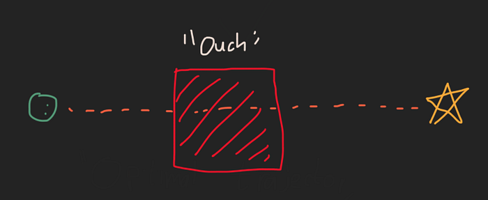
This works, but has some slight flaws. Imagine you have a pit of death™ between you and the fridge. Our “find the minimal length” algorithm would run you right through that, which I think you might agree is not truly optimal.

A potentially better cost function (and what I mainly used in my Starship landing code) is based off of “Effort”. Say that it takes you a 1 point of effort to move a step forward on the floor, and it takes you 1000 points of effort to go through the pit of death™. This better matches what we consider to be optimal vs not optimal:

Finally, constraints:
Few optimization problems are complete without a good set of constraints, here’s some “logical” ones for our get-to-the-fridge-with-minimal-effort problem :)

Extra resources:
This is the heart of what trajectory optimization is; Optimize a trajectory between points by minimizing some cost function, and holding a set of constraints. Here’s some good resources that go way more into depth on the math side of this:
Introduction to Trajectory Optimization, Mathew Kelly, Youtube.
Landing a rocket! — The code
Now onto the fun stuff. There are some amazing libraries out there that churn through equations and do the heavy lifting of optimization, so the real “art” lies in asking the right question to the solver. If you want to follow along line by line (I promise its not that many lines) or fiddle around with it, here’s a link to a collab notebook that lets you run this all in your browser:
The library I am using to run my optimization is CasADI: https://web.casadi.org/
The Trajectory:
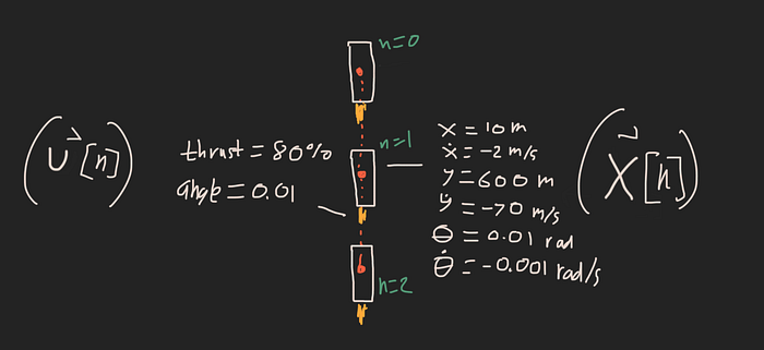
Time was sliced up into 0.04s chunks and variables for the rockets state and control state were generated at each step. This results in a bunch of discrete points along the path that are easier to work with then trying to come up with a closed form solution for the entire thing (pretty much impossible).

Rocket state vector: x[n] = [x, x_dot, y, y_dot, theta, theta_dot]
Control state vector: u[n] = [thrust_mag, thrust_angle]

(0.04s was picked because it results in 1:1 playback at 25 frames a second. Yes, I did in fact change the simulation timestep because 25 fps looks nice)
To find the number of timesteps, I manually increased the number until a feasible solution was found. There are ways of having the solver discover the minimum time trajectory on it’s own (mainly: letting it decide the timestep between points), but that gets harder to animate.
The Cost Function:

(all costs are sums of squares-> cost[0]² + cost[1]² + cost[2]² … and so on)
Minimize thrust output — Ideally you would like to use a little fuel on landing as possible.
Minimize TVC gimble angle — Moving your nozzle is effort, and ideally you want it to nominally be pointing downwards.
Minimize angular velocity — Seems like a bit of wild card, but I had a hunch that angular velocity / acceleration puts the largest amount of strain on the vehicle, so you would like to keep that as low as possible.
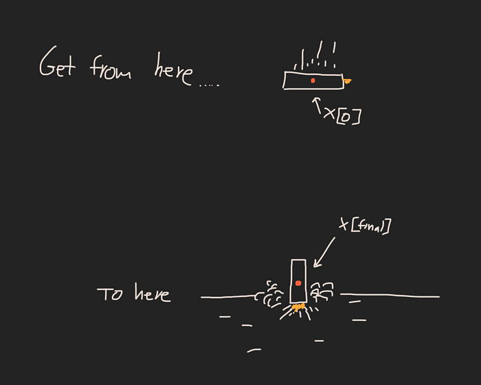
Constraint set 1: Initial and Final conditions

The initial condition is starting 1000m in the air traveling down at 80m/s, rotated 90 degrees.

The starting height and speed were taken from the SN9 data available at Flight Club: https://flightclub.io/result/2d?code=SN91
Constraint set 2: Dynamics

Each state timestep has to obey: x[n+1]-x[n] = f(x[n], u[n]) * dt
This is essentially the “don’t break physics” constraint. It is equivalent to a discrete time simulation of the rocket, the next state is equal to the current state + the derivative * dt. (Note: I used x_dot() instead of f() in the code because I think it makes it easier to read).

Vehicle constants and dynamics function:
g = 9.8
m = 100000 kg (guessed a nice round number between wet and dry mass. In reality, this would change as you used fuel, but I was going for simplicity over accuracy)
length = 50 meters
I = (1/12) * m * length² (inertia of a uniform rod)

(Note: this is a fairly poor discretization, and much better methods exist, such as collocation. However, this is the easiest and fastest way to write this out)
Constraint set 3: Variable Bounds
Thrust cannot go greater than the single raptor maximum, cannot throttle below 40%, and the thrust vector control cannot gimble beyond 20 degrees in each direction
Raptor max was taken from Wikipedia, the +-20 degrees was totally a guess, and I would love to know if there is more reliable data for this.

Optimize!
All that’s left to do is run it!

And that’s basically it, you call opti.solve(), which then goes and translates our problem into something that Ipopt (an open source optimization solver) can understand. After thinking for a bit, hopefully this message should arrive at the bottom of a tall stack of iteration prints:


The next bit of code uses matplotlib to make a nice animation, it takes a bit to generate all the frames but the result is quite nice.

So “what did we learn”?
While the near perfect track is probably mostly me getting lucky with my estimations for things, there’s some interesting stuff to pull out of it, mainly:
Starship is very very likely either following a pre-planned optimized trajectory, or running real time optimization to generate an optimal trajectory on the fly. (or a mix of both)
More than this, we can go a bit further and guess that their optimization cost function / “objectives” are very similar to ours: Minimize thrust, Minimize TVC angle and Minimize angular velocity. The track is almost uncanny at times, especially with how far it slides out both ways. (I always assumed that was overshoot, but it could just be the optimal path to the landing pad). This is also a fun analysis tool, I really want to go figure out some additional constraints that cause the landing failures of SN8 and SN9 (requires a bit of tweaking: the final state can no longer be a rigid constraint).
Why actually landing a rocket is much harder than this:
Its tempting to go “woah I just figured out how SpaceX lands their rockets!!”, but sadly, that’s not really true.
Once you have generated a physically possible trajectory that gets you where you want to go, there’s a whole host of things that you need to do to actually go follow that trajectory: state estimation, closed loop feedback control, dynamically updating that trajectory based on real time conditions… and many more that someone who is an actual aerospace engineer (which I am not) would know. Beyond that, these solvers take a long time to run, and online (real time) optimization is incredibly hard to pull off correctly and safely: one wrong input and your solver could just spit back “fail”, causing the thing to fall out of the sky.
Extra resources:
Edit: (since a bunch of people appear to be finding this): Here’s a link to Lars Blackmore’s website, the lead engineer working on Starship EDL (Entry, Decent and Landing) and the person behind the Falcon 9 landing techniques. His thesis and other publications have much more comprehensive overviews of how optimal control can be used in the EDL problem. http://larsblackmore.com/
Thanks!
Anyway, thanks for making it this far, hope you learned something. Feel free to reach out to me on twitter or email (thomas.godden at outlook.com) if you have questions.
